Creating Images with MATLAB
Ok, last article is a prerequisite for this one – so please go through that if you do not know the basics of how pixels are arranged in an image.
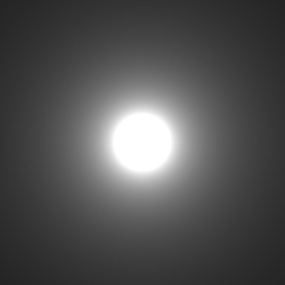
To start with, we are going to create a nice little ‘spherical light’ using basic maths and then proceed to create a ‘hypnotising’ animation using a little advanced maths – and all of this in MATLAB.
MATLAB looks at images as a matrix containing pixels, so manipulating them will be easy.
A basic jpg image will be seen as a height x width x 3 matrix, which means it’s a 3D matrix of three layers deep with each layer specifying a channel (Red, Green and Blue).
An indexed image (like a .gif for example) will be a 2D height x width matrix with an extra property called a ‘map’. The 2D matrix is called an intensity matrix which contains a grey scale version of the image. Whites are denoted by high values (1s if the matrix’s a double type, 255s if it’s a uint8 [unsigned integer – 8bit] type) and blacks by low values (0s). And of course the values in between denote different shades of grey. A map is another matrix (mx3 matrix, m variable and 3 = RGB) which associates each value in the grey scale matrix with a color. Hence you get a color image as a product. This method of imaging is used in heat imaging, where you just get the greyscale (intensity), and you map it with a predefined set of colors.
Let’s get started:
- Start by creating a 1000x1000 matrix (call it B) and fill it up with 0s. This matrix is later going to contain the image. (If you want, you can execute imshow(B) and see how the image looks like now – should be totally black)
- Start a loop in a loop with x and y as variables and in it, define a variable z which measures up the distance from the centre of the image
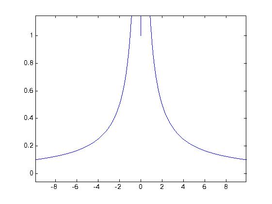
- To get the above effect, we are using the function |x-1|. The graph looks like this, with a central peak, which is what we want – a maximum in the middle and diminishing as we move away.

- To avoid any divide-by-zero errors, lets remove the case by using if statements
- To view the image, use ‘imtool(B, “InitialMagnification”,100)’ which sets the initial magnification to 100%
The code:
m = 1000;
B = zeros(m,m);
for y=1:m
for x=1:m
z=sqrt((m*.5-x)^2 + (m*.5-y)^2);
if z~=0
B(x,y)=(10/z);
else
B(x,y)=1;
end
end
end
imtool(B,'InitialMagnification',100);
If you change the value of the numerator in 10/z, you will be getting different intensities. A 100/z will fill out nicely and a 1/z will look like a dot.
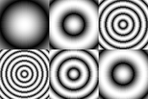
Yes, that was simple indeed. Now we’ll see how to achieve this animation using a similar technique:
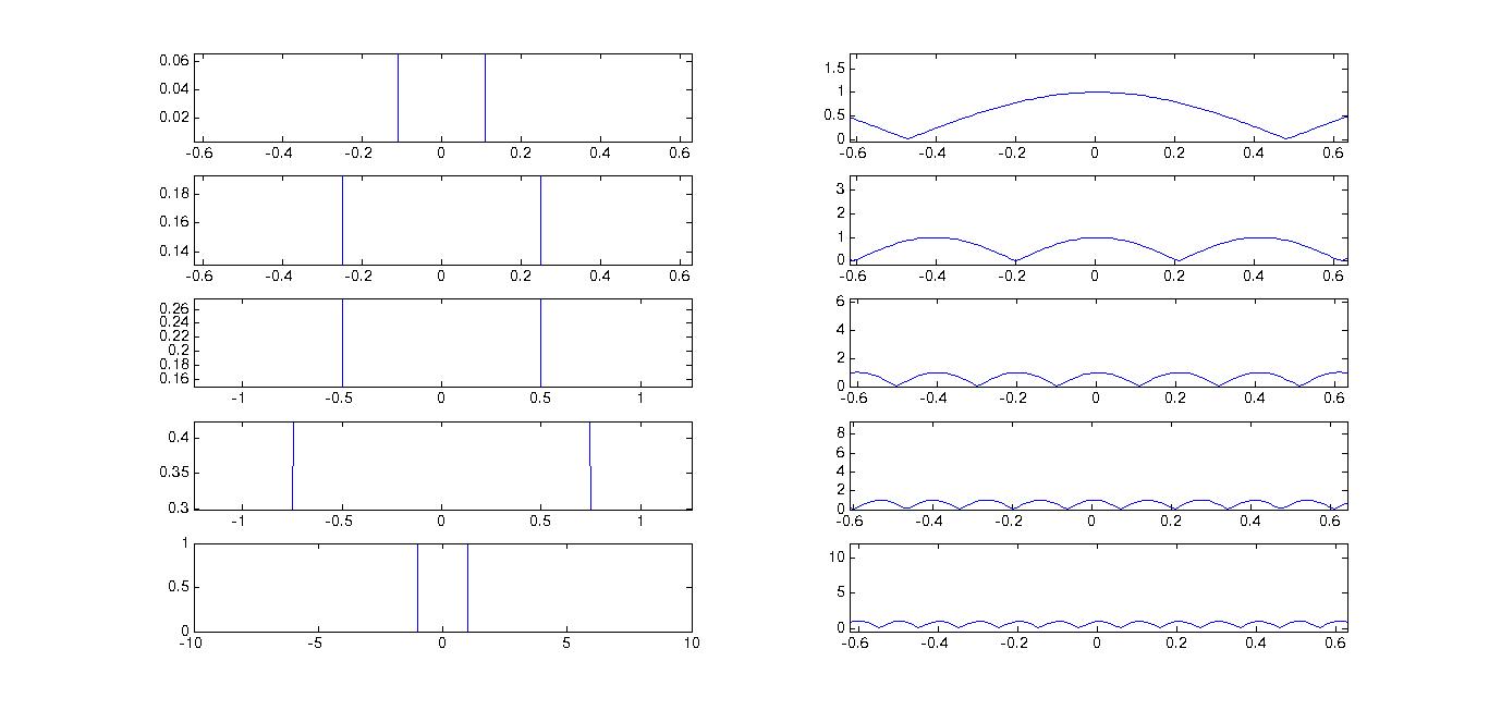
First, let’s examine some plots of Fourier transforms of a rect-function. The parameter changing here is the pulse width of the square function. And for each width, we obtain a different graph with different number of peaks in an interval. As the pulse width increases, the number of peaks increase. We are going to make use of this property in getting these frames.
m = 100;
B = zeros(m,m,1,8);
t=-10:0.01:10;
i=1;
for pulseW= [0.1,0.25,0.5,0.75,1]
y=(t>-pulseW&t<pulseW);
ft=abs(fft(y));
for y=(1):(m)
for x=(1):(m)
z=sqrt((m*.5-x)^2 + (m*.5-y)^2);
B(x,y,1,i)=((ft(round(z)+1000)));
end
end
i=i+1;
end
for i=6:8
B(:,:,:,i)=B(:,:,:,10-i);
end
[X map]=gray2ind(B,256);
mov = immovie(X,map);
imwrite(X,map,'anim.gif','gif','DelayTime',0.05,'LoopCount',Inf);
implay(mov);
Explaining the code:
- We are going to work with a smaller matrix as it is going to occupy less memory. Don’t try to work with huge ass matrices, your system WILL crash. Define B to be a 100x100x1x8 matrix. Why? The 100x100 is the size of the image, and the 1 is the number of channels, the 8 being the number of frames. This 4D matrix represents a multiframe image.
- Now defining the time interval from -10 to 10 with 2000 points in middle to get a proper transform.
- Next define the pulse widths in another matrix, pulseW.
- We are now going use this matrix to loop, to get the first five frames of the image. For each loop, we are using the pulse width from this matrix and get a Fourier Transform of the rect-function.
- Next, as done previously, create two loops with x and y and define z as the distance from the centre of the image. ‘ft’ contains the transform values. Offset it by 1000 to get values near zero. Put the value in in a pixel in B.
- After all these loops, we need to copy the 4th, 3rd and the 2nd frames into the 6th, 7th and 8th frames to get a smooth animation.
- The last few lines are to get the output properly. ‘gray2ind’ converts B which is a greyscale matrix into an index matrix (X) along with a map.
- ‘immovie’ creates a movie sequence from the multiframe image. To play the movie, we use ‘implay’.
- ‘imwrite’ is used to get the gif output. The parameters are set so that the frame rate is 20fps (i.e., 0.05s between each frame) and the animation goes on forever.
Thanks for reading!
The next episode will take a considerable time, and I didn't even plan a topic yet.


